Structural Smoothing
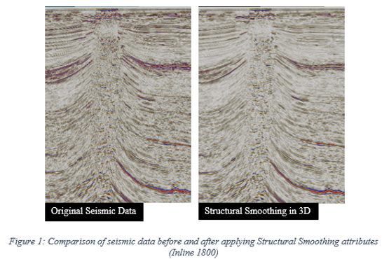
Figure 1 shows the original seismic data before and after applying structural smoothing attributes. The original seismic data looks more chaotic before applying the structural smoothing attributes but it became less chaotic after applying it. This helps us to ease our interpretation of our seismic data. From here we can see by using this attribute we can remove anomalies and noise from the seismic data and give us a clear view of any structure in the data.
Structural smoothing is used to increase the continuity of the seismic reflectors and it reduces the unnecessary noise by filtering out the artefacts of the real data. This attribute is very useful to increase the horizontal and vertical resolution to determine the local structure and stratigraphy.
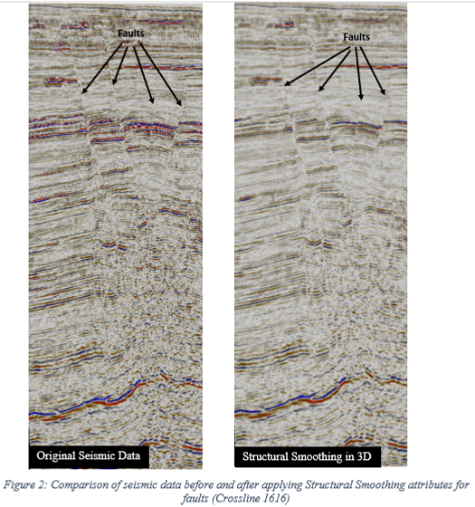
In Figure 2, before we apply the attribute, the fault is visible but more chaotic. After we apply structural smoothing, the whole data is less chaotic causes the fault to become more visible and easier for interpretation.
Structural smoothing has 3 display which are plain, dip guided and dip guided with edge enhancement. Plain setting will result in running a regular Gaussian smoother. The dip-guided option will filter in the direction of the dipping in the seismic. When edge enhancement is selected two half filters will be run. First, the chaos in both filter will be calculated. Then, the filter with the least chaos will be Gaussian filtered. This results in visually enhanced edges.
Based from the figures above, slight difference among plain, dip guided and dip guided with edge enhancement have been noticed at the same value of Sigma X, Y, and Z at 1.5. The black circle shows the areas with differences that have been identified within these three methods.
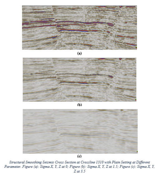
Sigma in structural smoothing shows that the size of this window can be defined independently for each orientation. A larger filter size will result in a smoother result reasonable values are in the range of 1.0-2.5 using sigma above 2.5 may significantly increase attribute calculation time. From the figure above, we can see that the best value which shows the best results is when Sigma X, Y and Z with value 1.5. For Sigma X, Y and Z at value 0, shows that the structural smoothing without its smoothing effect does not remove the noises efficiently but some of it is removed for Sigma X, Y and Z at value 1.5. Thus, we can see clearly structures like faults in the data. But applying too much of structural smoothing, Sigma X, Y and Z at value 3.5, the data is too smooth until it is hard for us to interpret it.